Highlights of Part 1 :

Ms. Dyuti Lal spoke and presented some of the important highlights of the implementation on how AI/ML can typically be categorized as aiding with one or more of the following: Keeping Well, Early Detection, Diagnosis, Decision-Making, Treatment, Research, etc along with few interesting case studies at Machine Conference 2019, Singapore.

In Part 1 we discussed about what is AI/ML and deep learning, its use cases, impact of AI in healthcare, its branches, functional requirement, key factor for AI to work and challenges to tackle. In this part we will be discussing on different case studies that was discussed during MachineCon 2019, Singapore.

The Machine Conference is an exclusive gathering of Analytics & Data Science Leaders in Asia by Analytics India Magazine.

Click here for Part 1

Data Description:

The dataset contains the following columns:

Description	Variable	Type
age	age in years	continuous	int
sex	1 = male, 0 = female	categorial	int
cp	chest pain type: 1: typical angina, 2: atypical angina, 3: non-anginal pain, 4: asymptomatic	categorical	int
trestbps	resting blood pressure in mm Hg	continuous	float
chol	serum cholestoral in mg/dl	continuous	float
fbs	fasting blood sugar > 120 mg/dl: 1 = true, 0 = false	categorial	int
restecg	0: normal, 1: having ST-T wave abnormality, 2: left ventricular hypertrophy	categorial	int
thalach	maximum heart rate achieved	continuous	float
exang	exercise induced angina (1 = yes; 0 = no)	categorial	int
oldpeak	ST depression induced by exercise relative to rest	continuous	float
slope	the slope of the peak exercise ST segment: 1: upsloping, 2: flat, 3: downsloping	categorial	int
ca	number of major vessels: (0-3) colored by flourosopy	continuous	int
thal	3: normal, 6: fixed defect, 7: reversable defect	categorial	int
target	diagnosis of heart disease: (0 = false, 1 = true	categorial	int

Correlation Between the Variables:

It’s easy to see that there is no single feature that has a very high correlation with our target value. Also, some of the features have a negative correlation with the target value and some have positive.

Understanding the Data:

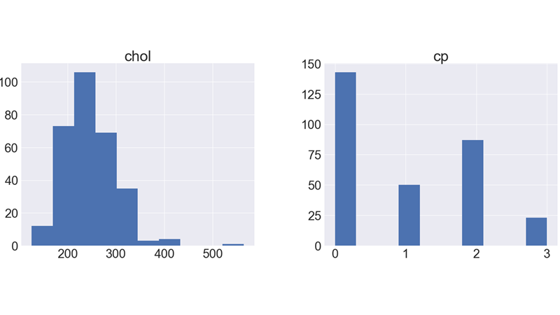
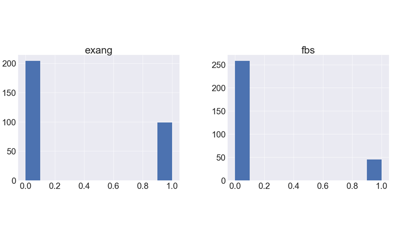
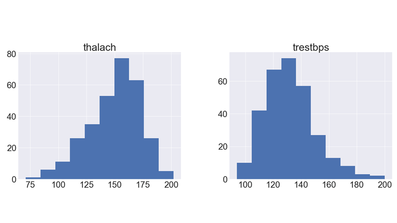
It shows how each feature and label is distributed along different ranges, which further confirms the need for scaling.

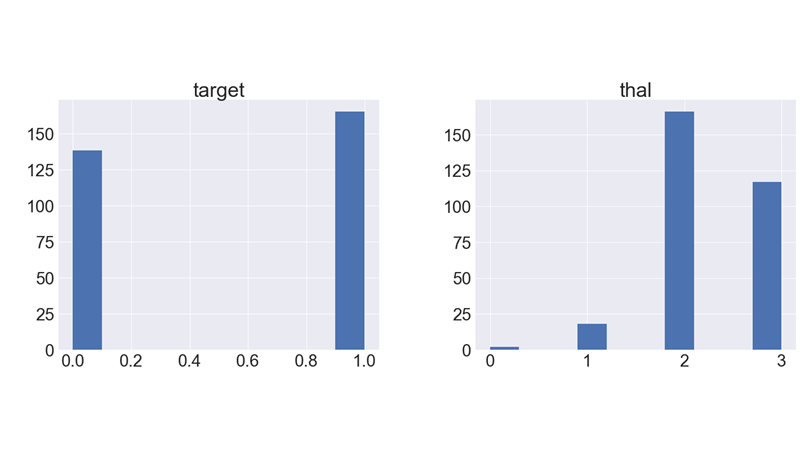
Target Variable:

Our target labels have two classes, 0 for no disease and 1 for disease.

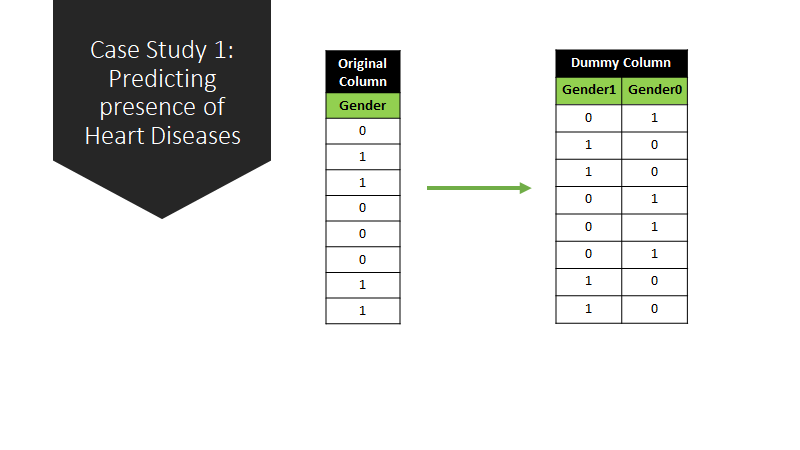
Data Processing

To work with categorical variables, we should break each categorical column into dummy columns with 1s and 0s.

Next, we need to scale the dataset for which we will use the StandardScaler. The fit_transform() method of the scaler scales the data and we update the columns.

Splitting Data to Train & Test

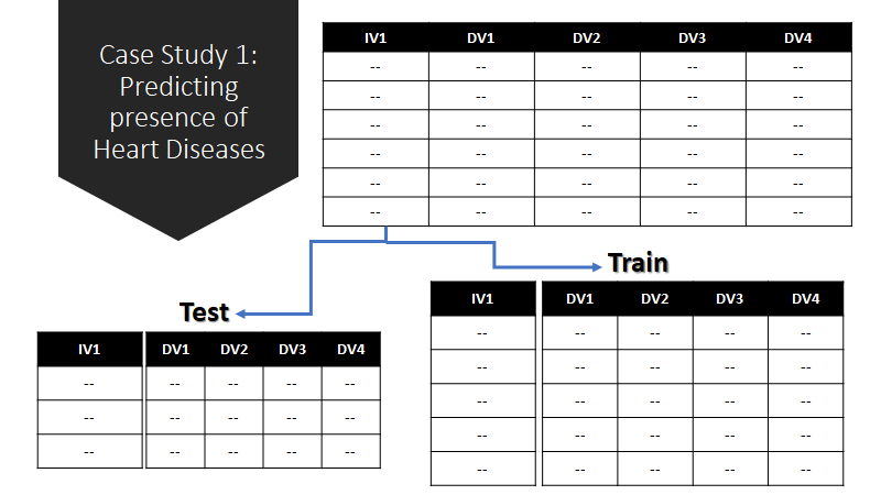
We have split the dataset into train as 70% and test as 30%.

We can begin with training our models.

Logistic Regression Model:

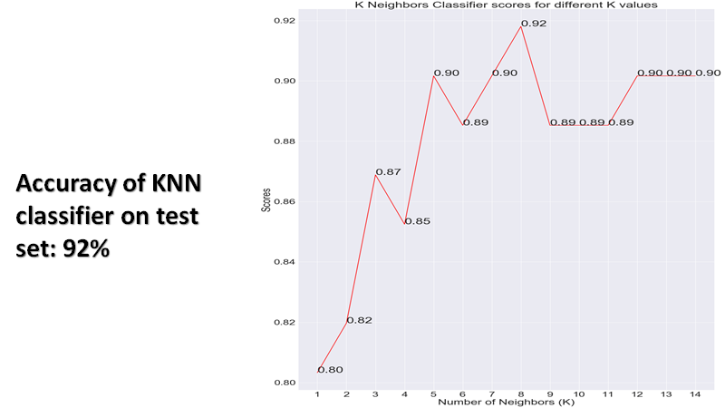
K N N Classifier:

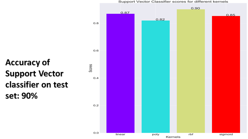
Support Vector Classifier:

Decision Tree Classifier:

Random Forest Classifier:

Data Description:

• There are 699 rows in total, belonging to 699 patients
• The first column is an ID that identifies each patient.
• The following 9 columns are features that express different types of information connected to the detected tumors. They represent data related to: Clump Thickness, Uniformity of Cell Size, Uniformity of Cell Shape, Marginal Adhesion, Single Epithelial Cell Size, Bare Nuclei, Bland Chromatin, Normal Nucleoli and Mitoses.
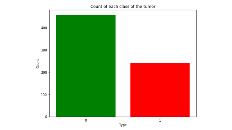
• The last column is the class of the tumor and it has two possible values: 2 means that the tumor was found to be benign. 4 means that it was found to be malignant.

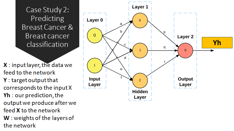
Data Processing:

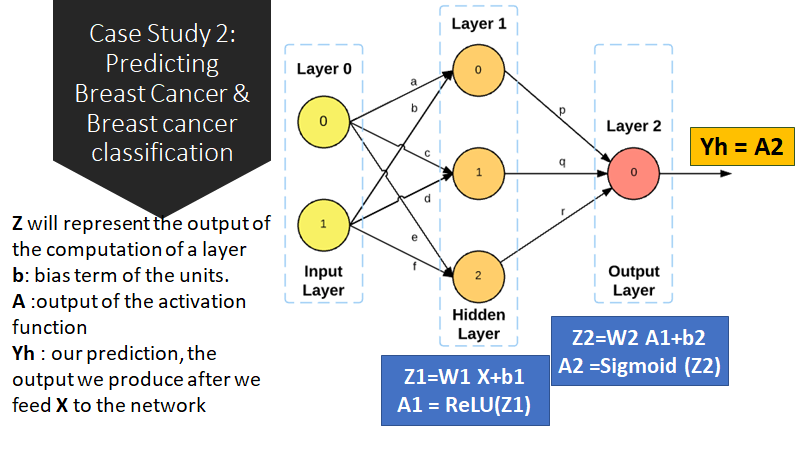
The benign and malignant classes are identified with the digits 2 and 4. The last layer of our network outputs values between 0 and 1 through its Sigmoid function. Furthermore, neural networks tend to work better when data is set in that range, from 0 to 1. We will therefore change the values of the class columns to hold a 0 instead of a 2 for benign cases and a 1 instead of a 4 for malignant cases. 

We also proceed to eliminate all rows that hold missing values.

Data normalization is a key first step within the feature engineering phase of deep learning processes.

Normalizing the data means preparing it in a way that is easier for the network to digest.

Splitting Data to Train & Test:

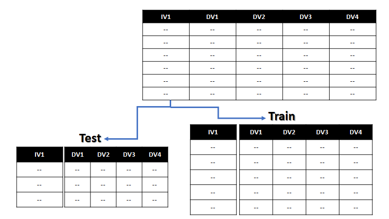
We have split the dataset into train as 70% and test as 30%.

We can begin with training our models.

Building Model using Tensor Flow

def build_model():
model = keras.Sequential([
layers.Dense(9, activation=tf.nn.sigmoid, input_shape= [len(train_x.keys())]),
layers.Dense(64, activation=tf.nn.relu),
layers.Dense(64, activation=tf.nn.relu),
layers.Dense(2, activation=tf.nn.sigmoid),
#layers.Dense(1)
])

model.compile(loss=’sparse_categorical_crossentropy’,
optimizer=’adam’,
metrics=[‘accuracy’])
return model